In Search of Lost Alpha

Summary

In this post I ask a practical question: in a constrained multi-asset portfolio, how much does the estimation machinery actually determine the result?

I test one Black–Litterman implementation across three asset universes, three estimation windows, two covariance estimators, two rebalancing frequencies, two transaction-cost assumptions and three tracking-error budgets. Within each specification, the Black–Litterman model is run at ten settings that progressively increase the weight placed on trailing sample returns relative to the equilibrium prior. Minimum variance, equal risk contribution and equal weight allocation methods provide controls.

The full experiment contains 216 specifications and 2,808 method-runs over a common ETF history from December 2007 to October 2025.

Three results dominate.

First, the tracking-error constraint determines the scale of the active portfolio. Once the Black–Litterman view weight is moderately high, further increases have almost no effect on realised tracking error. The confidence setting mostly determines how quickly the optimiser reaches the constrained region.

Second, the investment universe matters at least as much as the estimation method. Median information ratio for Black–Litterman is −0.08 in the six-asset universe, +0.12 with fifteen assets and +0.09 with 33 assets. More breadth helps initially, but the widest universe does not produce the best optimised result.

Third, the incremental return from estimation is difficult to separate from sampling noise. A block bootstrap for a representative wide-universe (of 33 assets) configuration produces an information ratio of 0.155 with a 95% interval of [−0.233, +0.561].

The controls are also informative. Minimum variance and equal risk contribution have negative benchmark-relative information ratios throughout this experiment, largely because their realised betas are well below the policy portfolio. Equal weighting performs very differently: it is poor in the six- and fifteen-asset universes but exceptionally strong with 33 assets.

This is not an argument against optimisation. In fact, the most important decisions are made before the optimisation even starts: how much active risk it is allowed to take and what opportunity set it is given. Fine tuning the estimation layer has a smaller effect.

The problem with standard optimiser tests

Portfolio optimisation is unusually easy to test unfairly.

One common problem is to rank benchmarked portfolios by Sharpe ratio. A minimum-variance portfolio can improve its Sharpe ratio simply by taking substantially less equity risk than the policy portfolio. That may be a useful portfolio, but it is not evidence that the optimiser has added benchmark-relative return.

For that reason, the main metric here is information ratio:

Alpha and beta relative to the policy portfolio are reported alongside it.

A second problem is dimensionality. Covariance estimation with 6 assets and roughly 63 to 252 daily observations is a different problem from estimation with 33 assets. At the shortest window in the wide universe, the observation-to-dimension ratio is only 63/33 or 1.91. The sample covariance remains full rank, but it is poorly conditioned.

A third problem is unconstrained optimisation. Institutional portfolios normally operate relative to a policy portfolio and within explicit active-risk limits. Testing an unconstrained optimiser therefore answers a different question from the one most benchmarked mandates face.

The experiment is designed around those three issues.

Experimental design

Benchmark-relative risk

Black–Litterman and minimum variance are subject to an ex-ante tracking-error constraint:

with annualised budgets of 1%, 2% and 4%.

The constraint uses the covariance estimate available at the rebalance date. Realised tracking error reported later is therefore not expected to equal the nominal budget exactly.

The fixed policy portfolio and equal weight are analytic controls. The equal-risk-contribution (ERC) implementation is unconstrained and unlevered, so its risk level can differ materially from policy.

Three investment universes

The portfolios contain 6, 15 or 33 assets, but each expresses the same strategic stance: 60% equity and 40% fixed income, allocated across six sub-classes: US equity, developed ex-US equity, emerging markets, government and agency debt, US credit, and real assets. What changes across the universes is the granularity of implementation within the asset roles.

The core universe contains six liquid ETFs: SPY, EFA, EEM, IEF, LQD and TIP – one instrument for each role and a portfolio a generalist investor could plausibly hold.

The broad universe expands to fifteen assets. US equity is split into large and small cap, the Treasury allocation is spread across SHY, IEF and TLT, and the opportunity set adds high yield, REITs and commodities while preserving the same six strategic roles.

The wide universe contains thirty-three assets. A single US equity allocation is replaced by the nine S&P sector SPDRs, rates are represented by a seven-instrument curve that also includes international sovereign bonds and agency MBS, and real assets are separated into gold, silver and broad commodities.

Within each strategic role, weights are divided equally across its constituent instruments rather than market-cap weighted. The role weights themselves are unchanged across the three universes. The experiment therefore increases the number of securities and the dimensionality of the estimation problem without intentionally changing the portfolio’s strategic exposure.

This lets me separate two questions that are usually mixed together: whether a richer opportunity set gives the optimiser more useful choices, and whether the resulting increase in estimation difficulty offsets that benefit.

The Black–Litterman dial

The Black–Litterman implementation starts from reverse-optimised equilibrium returns calibrated to an implied Sharpe ratio of 0.35.

A parameter denoted τ controls the weight placed on the trailing sample-mean view relative to that prior. τ=0 reproduces policy and increasing τ places progressively more weight on recent realised returns.

The settings for τ parameter are: 0, 0.01, 0.025, 0.05, 0.10, 0.25, 0.50, 1.00, 2.50 and 5.00.

Estimation and rebalancing

At each rebalance date, the optimiser estimates expected returns and covariance from the daily returns available up to that point. The lookback window is 63, 126 or 252 trading sessions; daily moments are then scaled to the 21-session investment horizon.

Scaling daily moments provides substantially more observations but it comes with the approximation trade-off. Scaled daily volatility overstates realised horizon volatility by roughly 21% for equities and 4% for Treasuries. Stock/bond correlation is approximately −0.29 using daily observations and −0.06 at the holding horizon.

The covariance estimate is calculated in two ways: the ordinary sample covariance and Ledoit–Wolf shrinkage. The latter regularises the sample estimate by pulling it toward a more stable target, reducing the influence of noisy pairwise correlations. The distinction should matter most when the amount of data is small relative to the number of assets. In the 33-asset universe with a 63-session window, the observation-to-dimension ratio is only 1.91. Comparing the two estimators across the grid therefore lets me test whether a more stable covariance estimate helps as the estimation problem becomes harder.

Once the estimates are formed, the portfolio is optimised and rebalanced. The rebalances happen at the end of 21-trading day blocks so every holding period contains the same number of days. The grid also tests a lower-frequency rebalance rule of 63 days, allowing me to separate the effect of changing estimates from the cost of acting on them more often.

Once the new weights are set, they drift with asset returns until the next rebalance. Transaction costs of 10 bp and 25 bp are applied to the turnover between end-of-period drifted weights and the new target weights.

The complete spec grid

The experiment contains:

3 universes × 3 estimation windows × 2 covariance estimators × 2 rebalancing frequencies × 2 cost settings × 3 tracking-error budgets = 216 specifications.

Each specification contains 13 methods: ten Black–Litterman settings, minimum variance, equal risk contribution and equal weight. That generates 2,808 method-runs. Dispersion in results should be interpreted as sensitivity to specification choices as the runs aren’t independent because they use the same underlying history.

1. The budget sets the scale

The clearest result appears when realised tracking error is plotted against the Black–Litterman view-weight parameter. In the 33-asset universe, realised tracking error rises initially and then flattens:

τ	1% ex-ante budget	2% ex-ante budget	4% ex-ante budget
0	0.00	0.00	0.00
0.01	1.14	1.31	1.33
0.025	1.41	2.15	2.41
0.05	1.42	2.68	3.33
0.10	1.42	2.76	4.14
0.25	1.42	2.77	4.70
0.50	1.42	2.77	4.87
1.00	1.42	2.77	4.92
2.50	1.42	2.77	4.95
5.00	1.42	2.77	4.95

For the 1% and 2% budgets, little changes beyond about τ=0.10. At the 2% budget, for example, increasing τ fiftyfold from 0.1 to 5 increases median realised tracking error only by 0.01%.

That result tells us that the portfolio has saturated, but not why. Higher-τ portfolios might all be running into the tracking-error constraint, or they might simply have converged to the same active portfolio before the constraint is reached.

The rebalance-date diagnostics separate those effects.

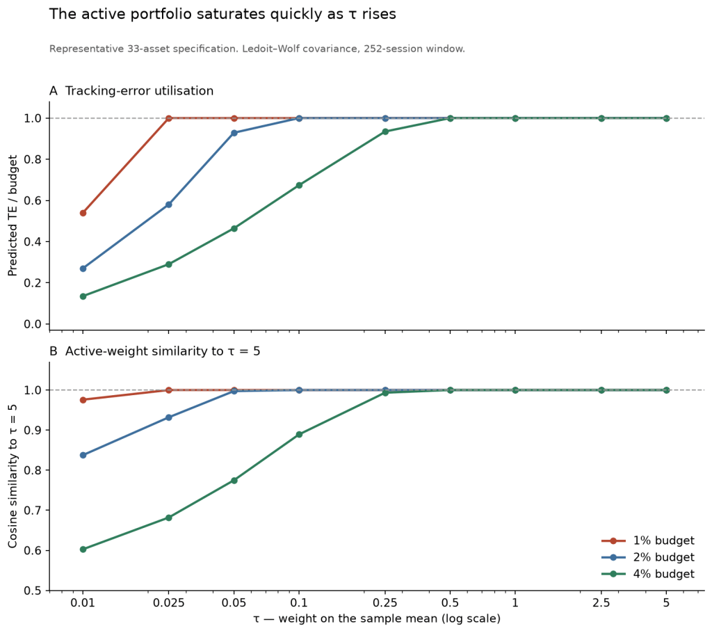
In the representative 33-asset specification, panel A shows ex-ante tracking-error utilisation: predicted tracking error divided by the permitted budget. Panel B shows cosine similarity between the active-weight vector at each τ and the corresponding τ=5 portfolio. A cosine similarity of 1 means the portfolios point in the same active-weight direction, although their magnitudes can differ.

The tight budgets saturate quickly. At the 1% budget, median utilisation reaches 1.00 by τ=0.025 and the active-weight direction is already identical to the τ=5 portfolio. At 2%, similarity is 0.997 by τ=0.05 and reaches 1.000 by τ=0.25, when the constraint is also binding on almost every rebalance date.

The 4% budget helps separate direction from scale. The active portfolio is effectively pointing in its final direction by τ=0.5, even though the tracking-error constraint is within 0.1% of its limit on only 65% of rebalance dates at that setting. Increasing τ further therefore adds little information about where the optimiser wants to go as the risk budget determines how far it is allowed to go.

The mechanism therefore can be described as: the expected-return signal settles quickly on an active direction, while the tracking-error budget limits the size of that active position. Once both have saturated, further increases in τ have almost no portfolio-level effect.

For governance, the implication is straightforward. The economically relevant range of τ is narrow. Beyond it, fine tuning the confidence setting changes little, while the tracking-error budget continues to determine how much benchmark-relative risk the portfolio can take.

2. Breadth determines how much active risk is useful

The optimiser behaves very differently as the opportunity set expands. The table below covers the 648 Black–Litterman runs with τ > 0 in each universe.

Universe	Assets	Median IR	IR Range	Specs with IR > 0	Median beta
Core	6	−0.079	[−0.17, +0.01]	27.5%	0.988
Broad	15	+0.121	[+0.01, +0.20]	76.4%	0.948
Wide	33	+0.085	[−0.03, +0.21]	68.8%	0.943

The Core universe gives the optimiser little to work with. Its median information ratio is negative and fewer than a third of specifications are positive.

Moving to fifteen assets changes the result materially. Median information ratio rises to +0.121 and more than three-quarters of specifications are positive. Expanding again to the Wide universe does not improve the median result: information ratio falls to +0.085.

Breadth therefore helps, but not monotonically. Going from six to fifteen assets creates useful additional choices. Going from fifteen to thirty-three adds still more choices, but also a harder estimation problem and more trading. In this sample, those costs offset some of the additional opportunity.

The amount of active risk that can be used productively changes with the universe as well:

Ex-ante TE budget	Core	Broad	Wide
1%	−0.040	+0.203	+0.034
2%	−0.053	+0.066	+0.123
4%	−0.113	+0.075	+0.140

The pattern is clearest at the extremes. In the six-asset universe, allowing more deviation makes performance steadily worse. In the thirty-three-asset universe, the ordering reverses: the 4% budget produces the highest median information ratio. The fifteen-asset universe does best with the tightest, 1% budget.

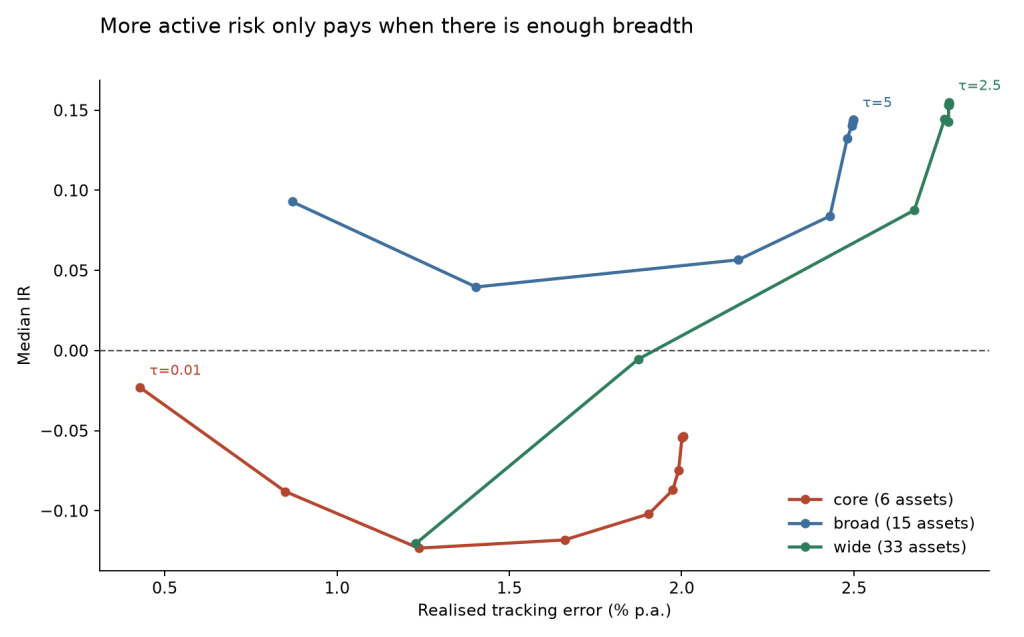
The same interaction appears when realised tracking error is plotted against information ratio as τ increases. In core, moving further from policy does not improve the result. Broad remains positive over a useful range of active risk. Wide benefits from greater deviation before performance levels off.

This matters because a tracking-error budget has no useful interpretation in isolation. A 4% budget may be sensible when the optimiser has thirty-three instruments through which to express a view and damaging when it has only six. A narrow universe with a loose risk budget gives the optimiser more freedom without giving it more independent opportunities.

Median betas remain between 0.94 and 0.99 for the Black–Litterman runs, so these differences are not primarily the result of large changes in market exposure.

The practical conclusion is not that wider universes are always better, or that tighter budgets are always safer. Breadth and active-risk budget need to be chosen together. The opportunity set determines what the optimiser can do; the budget determines how much room it has to do it.

3. Shrinkage does not help where expected

One reason for varying the covariance estimator was to test a simple prediction: Ledoit–Wolf shrinkage should help most when the number of observations is small relative to the number of assets.

The results do not support that prediction.

Estimation region	IR change from Ledoit–Wolf
Fewer than 4 observations per dimension	−0.009
At least 4 observations per dimension	+0.051
Hardest point: 63/33 = 1.91	−0.008

At the hardest point in the grid, shrinkage produces essentially no improvement there. More broadly, its median contribution is slightly negative when the ratio is below four and positive in the easier estimation region.

That is the opposite of what I expected. It does not mean shrinkage is ineffective in general. In this experiment, its theoretical advantage in the most data-constrained settings does not translate into better realised benchmark-relative performance.

One possible explanation is that when the covariance estimate becomes sufficiently unstable, portfolio constraints limit the effect that differences between estimators can have on the final allocation.

4. Simple controls are hard to beat

The control portfolios help separate two different questions: whether an optimiser produces a sensible portfolio, and whether it adds value relative to the policy portfolio.

Minimum variance and equal risk contribution perform poorly on the second test.

Runs	Positive IRs	Median IR	Median beta
432	0	−0.462	0.624

None of the 432 runs has a positive information ratio. The median beta of 0.624 explains much of the result: these portfolios take substantially less policy risk.

That does not make minimum variance or ERC bad portfolios. It means that if they are used unlevered, they answer a different question. They reduce absolute risk rather than trying to improve returns relative to the policy portfolio. Information ratio makes that distinction explicit. Only 0.2% of the runs produce an alpha t-statistic above 2 in absolute value.

Equal weighting is the more demanding control because it uses the same opportunity set without estimating either expected returns or an optimal covariance-based allocation.

In the Wide universe, it is the strongest method in the study:

Median information ratio	+0.685
Positive specifications	72 of 72
Median alpha	+0.52%
Median alpha t-statistic	+2.65
Specifications with alpha t > 2	100%
Median beta	1.023
Median realised tracking error	0.94%

The result is not a general case for equal weighting. In the Broad universe its information ratio is about −0.42, and in the six-asset universe about −0.78. Its success appears only when the opportunity set is sufficiently broad.

That makes the result more useful, not less. In the Wide universe, much of what looked like an optimisation opportunity was also available from a simple diversification rule. Equal weight achieved a substantially higher information ratio while taking less active risk: median realised tracking error was 0.94%, compared with about 2.59% for the Black–Litterman runs.

The comparison is not perfectly risk-matched but it does establish an important benchmark for practice: before attributing value to the estimation machinery, check whether a simple rule on the same universe captures the same opportunity more efficiently.

In this experiment, the wide-universe optimiser does not clear that bar.

5. Trading costs do not explain the main result

Black–Litterman (B-L) turns over roughly 140% a year compared to 10% for the policy portfolio. So implementation costs are a plausible explanation for weak performance. The backtest therefore applies one-way trading costs and asks a practical question: at what cost does each strategy’s information ratio fall to zero?

Method	IR at 0bp	3bp	10bp	25bp	Break-even
B-L, Core	+0.052	+0.033	−0.023	−0.145	7.6bp
B-L, Broad	+0.234	+0.213	+0.163	+0.030	29.0bp
B-L, Wide	+0.264	+0.211	+0.147	−0.014	23.7bp
EW, Wide	+0.686	+0.686	+0.685	+0.684	>50bp

The six-asset optimiser has little room for execution costs. Its estimated break-even is only 7.6bp one way. The broader universes are more robust: broad remains positive to about 29bp and wide to about 24bp.

That distinction matters because it rules out a simple explanation for the breadth result. The optimiser is not failing in core merely because a more diversified portfolio trades more. Even before costs, Core has only a small positive information ratio, while Broad and Wide start materially higher.

Equal weight is the clearest control. Its information ratio barely changes across the cost sweep because turnover is low. More importantly, it already outperforms the optimised methods at zero cost. Trading costs therefore widen the gap but do not create it.

The conclusion is straightforward: costs matter, but they do not overturn the main comparisons in the study. In the broader universes the optimiser survives a substantial cost burden, while equal weight retains its advantage even when trading is assumed to be free.

6. Historical uncertainty remains large

The 216 specifications vary multiple parameters but they don’t provide 216 independent tests of the strategy.

Agreement across the grid therefore tells us that a result is robust to modelling and implementation choices. It does not tell us how reliably the result would repeat in a different historical period.

That distinction matters for the Black–Litterman results. A positive median information ratio across many specifications can arise because the underlying signal genuinely has a positive expected return, but it can also arise because the common sample happened to favour that signal. Changing the estimation window or covariance estimator does not create a new history.

To measure that second source of uncertainty, I use a circular block bootstrap on a representative wide-universe Black–Litterman specification. Twelve-block resampling windows preserve some of the serial dependence in returns, and the strategy is evaluated across 1,000 bootstrap histories.

Information ratio: 0.155
95% bootstrap interval: [−0.233, +0.561]

The interval is wide and confidently crosses zero threshold. For that configuration, the available history does not provide enough evidence to distinguish the estimated active return from sampling variation.

This does not contradict the earlier robustness results. The specification grid asks whether the conclusion survives reasonable changes to the way the strategy is implemented. The bootstrap asks how uncertain the result remains because we have observed only one sequence of market returns.

For practitioners, both matter. A result that disappears when the lookback window changes is fragile in one sense. A result that survives every such choice but has a wide bootstrap interval is fragile in another.

The evidence here is strongest on the first question. The main findings – rapid saturation of the confidence setting, the interaction between breadth and active-risk budget, and the strength of the simple controls – recur across many specifications. The evidence that Black–Litterman contributes a positive expected active return is much weaker.

What I take from the experiment

The experiment does not show that portfolio optimisation is useless. It shows that some decisions matter much more than others.

The first is the active-risk budget. In the Black–Litterman runs, increasing the confidence setting initially changes the portfolio, but the effect fades quickly. The active direction converges, and the tracking-error constraint then determines how much of that position can be expressed. Fine tuning the confidence parameter beyond that point adds little.

The second is breadth. Moving from six to fifteen assets materially improves the opportunity set, but moving from fifteen to thirty-three does not improve the optimised result further. The useful amount of active risk also changes with the universe: tight budgets work best in narrower opportunity sets, while the widest universe benefits from more room to deviate.

The estimation layer matters less than I expected. Ledoit–Wolf shrinkage does not improve realised performance where the covariance problem is hardest, despite a strong theoretical reason to expect it to. That is a useful negative result. More sophisticated estimation does not automatically translate into a better portfolio once constraints and implementation choices are imposed.

The simple controls are equally important. Minimum variance and ERC are poor benchmark-relative substitutes for the policy portfolio when left unlevered, largely because they take much less policy risk. Equal weight presents a harder challenge. In the 33-asset universe it beats every optimised method in the study while taking less active risk and turning over far less. That result does not generalise to the narrower universes, but it does show that some of the apparent benefit of optimisation in the wide universe comes from breadth itself rather than from estimation.

Trading costs do not change that interpretation. Black–Litterman remains viable at plausible execution costs in the broader universes, but equal weight already has the advantage at zero cost. Costs matter for implementation, not for explaining the main ranking of methods.

The final qualification is statistical. The grid contains 216 specifications, but they all draw on the same history. Their agreement shows robustness to modelling choices; it’s not independent confirmations of an expected return. The bootstrap analysis clarified that the estimated Black–Litterman edge remains too uncertain to separate confidently from sampling variation.

For a practitioner, I would therefore put the decisions in this order: choose the opportunity set, set the active-risk budget, benchmark against simple rules, and only then spend time refining the estimator. The optimiser still matters, but it operates inside choices that have already determined much of what the portfolio can become.