Key takeaways
- I test two versions of buying the dip from 1962 to 2025. One keeps 10% in Treasury bills and the other starts at 60/40 and raises equities to 90%. Both deploy after a 20% market drawdown and reset when the market reaches a new high.
- Both dip buyers beat the static portfolios they started from, but they also held more equity on average and suffered deeper drawdowns. The cash version still finished behind 100% equities, while the bond version had a lower Sharpe ratio than 60/40.
- After matching the average equity exposure, timing added some return under the −20% rule. Allocation also mattered, so the result cannot be read as a pure reward for buying cheaply.
- The timing evidence is weak. The regression alphas are not statistically significant, the timing result turns negative with a −10% trigger, and the base test contains only twelve deployments. I would treat it as a result for this particular rule, not a general law about buying dips.
What does a dip buyer actually do?
Ask whether buying the dip beats buying and holding, and the intuitive answer – of course it does, you are buying the same thing cheaper – assumes that the discount is what does the work. It usually is not that simple.
A dip buyer who keeps a reserve is running two strategies stapled together. There is timing – buying after prices fall – but there is also allocation. Hold cash or bonds between selloffs and more stock after them, and over a full cycle the portfolio settles at some average equity weight. Timing is a claim about when to buy and allocation is simply how much equity risk the rule carried.
This question has been tested before. Nick Maggiulli gives an investor perfect knowledge of every future bottom and still finds that regular monthly investing wins in most 40-year windows. Benjamin Felix and Braden Warwick reach a similar conclusion across several national and global equity markets. Waiting reduces returns, while much of the apparent downside protection comes from the cash held before the trigger.
Bonini, Shohfi and Simaan formalise the rule and show how much the result depends on the starting market environment and the chosen dip size. AQR tests 196 variations and finds little reliable alpha after adjusting for average market exposure.
Most of this work treats dip buying as an entry decision: cash arrives, waits for a fall and then goes into stocks. Here the dry powder is already inside the portfolio – cash in a 90/10 allocation or bonds in a 60/40 one. It’s deployed after a 20% fall, rebuilt at the next high and used again. I compare each rule with a static portfolio holding the same realised average equity weight. The gap between them is the part attributable to timing rather than the allocation the rule happened to create.
The setup
I run a daily backtest using total returns. US equity and one-day T-bill returns come from the Ken French Data Library; the bond leg is a 10-year Treasury total-return series I build from FRED’s constant-maturity yield with the standard duration approximation, the same construction I have used before. The sample runs from January 1962 to July 2025, with dividends and interest reinvested and every portfolio starting at $1.
I test five portfolios:
- Equity buy-and-hold. 100% US equity market allocation.
- Static 90/10. 90% equity and 10% cash, rebalanced monthly.
- Static 60/40. 60% equity and 40% bonds, rebalanced monthly.
- Cash-reserve dip buyer. Starts at 90/10. When the market closes at least 20% below its prior high, it puts the whole cash reserve into stocks. At the next new high it rebuilds the 10% cash reserve.
- Bond-funded dip buyer. Starts at 60/40. On the same −20% trigger it increases equity allocation to 90%, funded from bonds, and resets to 60/40 at the next new high.
Each dip buyer also gets a static twin holding its realised average equity weight and rebalanced monthly. I use those twins below to separate allocation from timing.
How the portfolios behaved
Below are the dip buyers’ equity weights, with the market drawdown shaded in red.
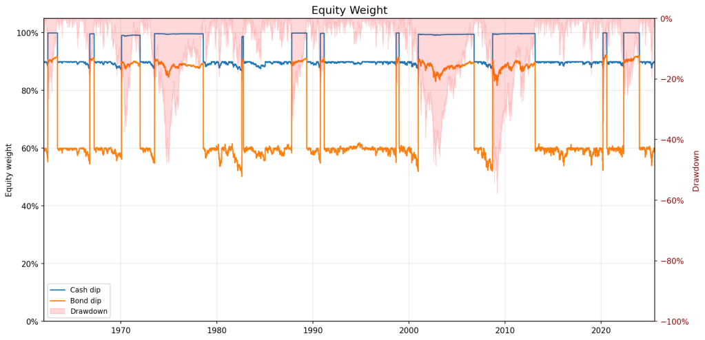
Whenever the market crosses the trigger, equity exposure rises – to 100% for the cash dip strategy and 90% for the bond dip one – into the 1970s bear market, Black Monday, the Dot-com bust, the GFC and COVID. The rule commits capital while prices are falling and other investors are selling, which is exactly why it feels disciplined.
The trigger often arrives too early in the worst bear markets. Once the market reaches the threshold, the reserve is spent in one go, leaving nothing for lower prices later in 1973–74, 2000–02 and 2008. From there, the strategy owns more equity until the market gets back to its previous high, however long that takes. A quick rebound is ideal. In a long bear market, it rides the rest of the decline with the maximum equity allocation.
It looks promising on the chart but the wealth paths are more ordinary.
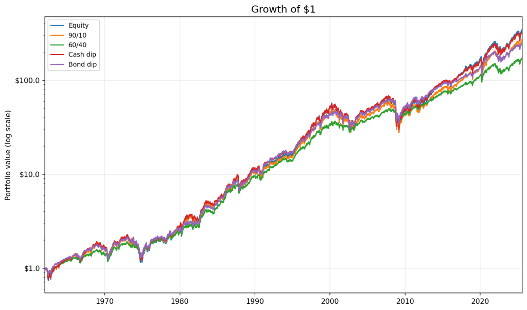
The CAGR ranking mostly follows equity exposure:
| Portfolio | CAGR | Vol | Sharpe | Max DD | Avg eq weight | Final wealth |
|---|---|---|---|---|---|---|
| Equity | 9.75% | 16.2% | 0.39 | −57.8% | 100.0% | $346 |
| Cash dip | 9.66% | 15.3% | 0.40 | −56.5% | 93.2% | $330 |
| Static 90/10 | 9.32% | 14.5% | 0.39 | −53.6% | 90.0% | $271 |
| Bond dip | 9.16% | 12.4% | 0.42 | −46.1% | 69.9% | $247 |
| Static 60/40 | 8.54% | 9.9% | 0.45 | −34.9% | 60.1% | $172 |
The cash-reserve strategy sits below 100% equity and above static 90/10, where its 93% average equity weight would put it. The bond-funded strategy sits between 60/40 and 90/10, where its 70% average weight would put it.
The cash-reserve dip buyer returned 9.66% a year against buy-and-hold’s 9.75%. Its timing was useful, but not useful enough to pay for the return forgone while the reserve stayed in T-bills. Both gains came with higher volatility and deeper drawdowns than the static starting portfolios. Static 60/40 still had the highest Sharpe ratio.
More equity or better timing?
The dip buyers do not keep the equity weights they start with. The cash strategy averaged 93.2% in equities rather than 90%; the bond strategy averaged 69.9% rather than 60%. A straight comparison with 90/10 or 60/40 therefore mixes two things: owning more stock and changing the weight after drawdowns. I want to separate them.
I do that in two ways. The first is a matched-weight decomposition. For each dip buyer I build a static twin with the same average equity weight and the same reserve asset. The twin rebalances monthly and never reacts to a drawdown. I then calculate:
- Total edge: dip buyer minus its original benchmark – static 90/10 for the cash strategy and static 60/40 for the bond strategy.
- Allocation: static twin minus the original benchmark.
- Timing: dip buyer minus the static twin.
The second method follows the basic regression approach used by AQR in Hold the Dip. I regress each strategy’s daily return above cash on the market’s daily return above cash. Beta estimates its market exposure; the annualised intercept is the return left after adjusting for that exposure. Newey-West standard errors provide the t-statistic.
The two methods answer slightly different questions. The matched-weight calculation splits the strategy’s CAGR and keeps the same cash or bond funding asset. The regression works with daily returns, controls for market beta and tells me whether the estimated alpha is distinguishable from zero. It is a single-factor model, so I use it rather as a cross-check.
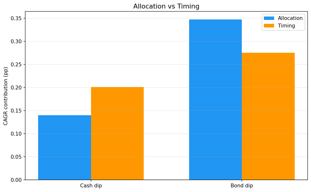
The chart shows the matched-weight split. The final three columns of the table show the regression result.
| Strategy | Baseline | Total edge | Allocation | Timing | Beta | Ann. alpha | t(alpha) |
|---|---|---|---|---|---|---|---|
| Cash dip | Static 90/10 | +0.34% | +0.14% | +0.20% | 0.95 | +0.13% | 1.10 |
| Bond dip | Static 60/40 | +0.62% | +0.35% | +0.28% | 0.74 | +0.57% | 1.22 |
For cash portfolios, the returns are 9.32% for static 90/10, 9.46% for the matched twin and 9.66% for the dip buyer. The first step contributes 0.14% from allocation; the second contributes 0.2% from timing. For bonds, the sequence is 8.54%, 8.89% and 9.16%, giving 0.35 points from allocation and 0.28 from timing.
Both regressions also produce positive estimates: 0.13% for cash and 0.57% for bonds. But the t-statistics are only 1.10 and 1.22, so neither is statistically significant. Both methods point in the same direction but the regression says the evidence is weak.
I call the matched-weight residual timing, but it is not a score for how close each purchase came to the bottom. It captures the whole path of moving equity exposure around the average weight. Nor is this a Sharpe decomposition: cash improved its Sharpe ratio only slightly relative to 90/10, while the bond strategy’s Sharpe fell relative to 60/40.
Why waiting is expensive
Waiting is expensive because equities have a positive expected return. A dip reserve held for the next drawdown spends much of its life earning bill rates while the market compounds without it. The strategy gives up part of the equity premium before it gets the chance to buy anything at a discount.
Dip buying also bets against momentum. It buys after declines, leaning against the market’s tendency to trend – the same point AQR makes in Hold the Dip. That does not make every purchase after a fall a mistake, but reversal is not a free source of return.
The weight chart shows why allocation and timing are easy to mix up. Raising equity exposure in a crash and holding it through the recovery also raises the strategy’s average equity weight. The static twin captures that part. Timing is only the return from moving around that average, not the return from carrying it in the first place.
The extra exposure shows up in the drawdowns. The cash-reserve strategy lost 56.5% at its worst, only slightly less than buy-and-hold’s 57.8%. The bond-funded strategy lost 46%, against 35% for static 60/40. That is what carrying more equity risk looks like on the way down.
How robust is the timing edge?
Each cell re-runs the matched-weight test with a different trigger and starting date. It shows the dip buyer’s CAGR minus the CAGR of its static twin, so a positive number means that changing the equity weight helped after controlling for average equity exposure.
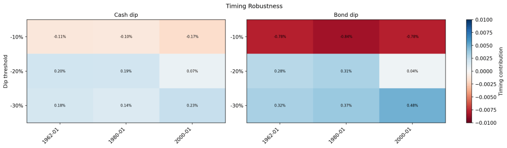
At −10%, timing is negative in every window: roughly −0.1 to −0.2 points for cash and about −0.8 for bonds. At −20%, it is positive over the full sample but nearly disappears when the test starts in 2000. At −30%, it is positive in every window.
A 10% rule is often triggered while the sell-off is still developing. A 20% or 30% rule enters later but ends up betting on a much smaller set of severe declines. The positive result therefore belongs to a narrow version of dip buying – late and rare – rather than to buying weakness in general. With so few deep drawdowns to learn from, it is hard to know whether the edge will repeat.
So, did buying the dip work?
Yes and no. In raw return terms, the cash strategy beat 90/10 by 0.34% a year and the bond strategy beat 60/40 by 0.62%. But neither portfolio took the same risk as its benchmark. Both held more equity on average and suffered deeper drawdowns. The cash strategy’s Sharpe ratio improved only slightly while the bond strategy’s fell.
No dip signal is needed to earn the allocation component. Holding roughly 93/7 instead of 90/10 accounts for 0.14 points in the cash strategy and holding 70/30 instead of 60/40 accounts for 0.35 points in the bond strategy. The part unique to moving the weight after drawdowns was 0.20 and 0.28 points respectively.
Whether that timing return will repeat is harder to say. The regressions point in the same direction, but their t-statistics are below significance threshold. Move the trigger to −10% and the timing residual turns negative in every window. There were only twelve −20% deployments in 63 years.
The US-only caveat is also worth flagging. One of the past century’s strongest equity markets makes waiting unusually expensive. A different market that spends decades bouncing around might be more suited for the strategy.
Finally, you can stick with the rule for this whole period and the cash dip strategy still finishes behind the investor who bought equities once and never looked again.


Leave a Reply